Advantages and Disadvantages of Linear Regression, its assumptions, evaluation and implementation

Problem Statement: Consider a real estate company that has a datasets containing the prices of properties in the Delhi region. It wishes to use the data to optimize the sale prices of the properties based on important factors such as area, bedrooms, parking, etc.
Objectives :
To identify the variables affecting house prices, e.g. area, number of rooms, bathrooms, etc.
To create a linear model that quantitatively relates house prices with variables such as number of rooms, area, number of bathrooms, etc.
To know the accuracy of the model, i.e. how well these variables can predict house price

3. Assumption in Linear Regression

Assumption - What is the assumption ?
Consequence - What will happen if particular assumption does not hold true ?
Check - Way to check particular assumption
Solution - Possible solutions so that assumptions hold true to implement LR.
Python Code - Python implementation to check the assumption on housing prices model

4. Understand use of Linear Regression in feature importance

5. Metrics to evaluate Regression

6. Advantages and Disadvantages of Linear Regression

7. Summary

1. Understanding Linear Regression

1.1 Analogy with real life Example

We come across many things where we apply simple linear equation to predict anything like suppose we know the price of 1 kg apples be it Rs 45 then to calculate for 10 kg apple we just follow a line equation

y = mx + c

here,
y = price of 10 kg apples
m = slope (price of 1 kg apples)
x = weight of apples(kg)
c = intercepts(default price of 0kg apples)

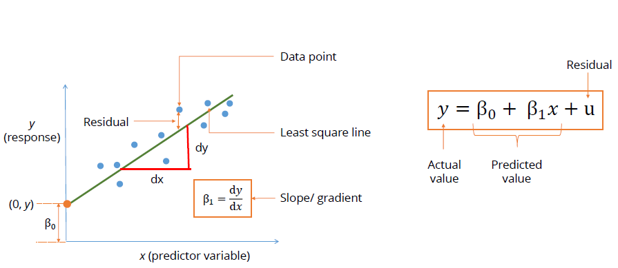
But when we buy zero apples we don’t have to pay anything so c(intercepts) here will be zero and the equation will be y=10x and this simple equation will help us to calculate any no of apples(in kg) and this is simple linear regression in terms of only one dependent variable but it becomes bit complex when we have multiple variables which affect our final answers .

1.2 Definition and types of Linear Regression

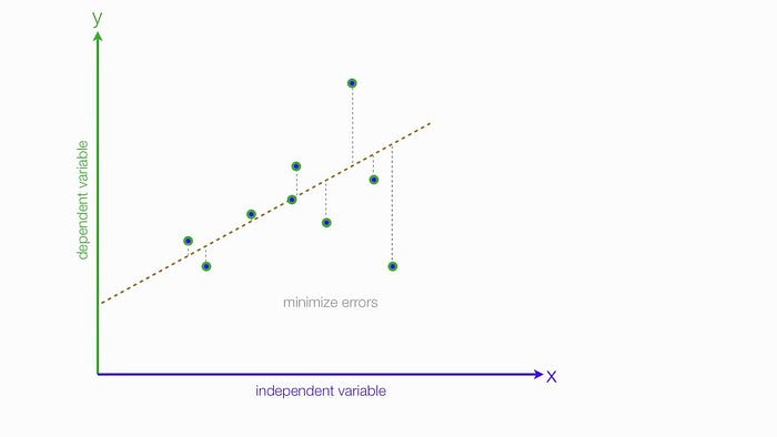
Linear Regression is a statistical method that allows us to summarize and study relationships between continuous (quantitative) variables. The term “linear” in linear regression refers to the fact that the method models data with linear combination of the explanatory/predictor variables (attributes). Linear regression models assume that the relationship between a dependent continuous variable Y and one or more explanatory (independent) variables X is linear (that is, a straight line). It’s used to predict values within a continuous range, (e.g. sales, price) rather than trying to classify them into categories (e.g. cat, dog). Linear regression models can be divided into two main types:

1.2.1 Simple Linear Regression

Simple linear regression uses a traditional slope-intercept form, where a and b are the coefficients that we try to “learn” and produce the most accurate predictions. X represents our input data and Y is our prediction.

Y = bX + a

1.2.2 Multivariable Regression

A more complex, multi-variable linear equation might look like this, where w represents the coefficients, or weights, our model will try to learn.

Y(x₁, x₂, x₃) = w₁ x₁ + w₂ x₂ + w₃ x₃ + w₀

The variables x₁, x₂, x₃ represent the attributes, or distinct pieces of information, we have about each observation.

2. Implementation in Python

For the purpose of this article we will consider uni-variate Linear Regression and House Price data for calculation of house prices based on various features like no of rooms , carpet area, location etc.

Data : You can Download the data from Kaggle — House Price — Data

Note : Here we are not going to deal with EDA and Feature engineering as the purpose of this article is to understand Linear Regression, its assumption, its use in Feature Selection and how to evaluate them.

2.1 Importing Packages and data

# Loading all the packages # Supress Warnings
import warnings
warnings.filterwarnings('ignore')# Import the numpy and pandas package
import numpy as np
import pandas as pd# Data Visualization
import matplotlib.pyplot as plt 
import seaborn as sns# Train test split
from sklearn.model_selection import train_test_split# Scaling 
from sklearn.preprocessing import MinMaxScaler# Importing RFE and LinearRegression
from sklearn.feature_selection import RFE
from sklearn.linear_model import LinearRegression# Metrics 
from sklearn.metrics import r2_score# Loading Housing data 
housing = pd.read_csv("Housing.csv")
housing.head()

2.2 Data Preparation

Converting all the categorical features to One Hot encoding

# List of variables to map
varlist =  ['mainroad', 'guestroom', 'basement', 'hotwaterheating', 'airconditioning', 'prefarea']# Defining the map function
def binary_map(x):
    return x.map({'yes': 1, "no": 0})# Applying the function to the housing list
housing[varlist] = housing[varlist].apply(binary_map)# Get the dummy variables for the feature 'furnishingstatus' and    # store it in a new variable - 'status'
status = pd.get_dummies(housing['furnishingstatus'])# Drop 'furnishingstatus' as we have created the dummies for it
housing.drop(['furnishingstatus'], axis = 1, inplace = True)# Add the results to the original housing dataframe
housing = pd.concat([housing, status], axis = 1)

2.3 Scaling

Scaling doesn’t impact your model for Simple Linear Regression.If we don’t have comparable scales, then some of the coefficients as obtained by fitting the regression model might be very large or very small as compared to the other coefficients and it will be difficult to interpret which feature is more important as it will be unit dependent. Example, Area in km sq. has coefficient 2 then coefficient of area in m sq. will be 1000 times i.e 2000 and can be falsely interpret area in m sq. is more effective. So, it is extremely important to rescale the variables so that they have a comparable scale. Therefore, it is advised to use standardization or normalization so that the units of the coefficients obtained are all on the same scale. As you know, there are two common ways of rescaling:

Min-Max scaling
Standardisation (mean-0, sigma-1)

This time, we will use MinMax scaling.

# Using MinMaxScaler 
scaler = MinMaxScaler()# Applying scaler() to all the columns except the 'yes-no' and      # 'dummy' variables
num_vars = ['area', 'bedrooms', 'bathrooms', 'stories', 'parking','price']# Fitting MinMaxScaler on train and test data 
housing[num_vars] = scaler.fit_transform(housing[num_vars])

2.4 Training and Testing Split

Splitting the data into 70:30 ratio for training and testing set

#Dividing into X and Y sets for the model building
y = housing.pop('price')
X = housing# We specify this so that the train and test data set always have   # the same rows, respectively
np.random.seed(0)
X_train, X_test, y_train, y_test = train_test_split(X, y, test_size=0.30, random_state=42)

2.5 Linear Regression Model fitting and Selecting Important Features

Fitting Linear Regression model and Selecting only 6 important Features based on beta coefficient and significance for our prediction

# Fitting Linear Regression model
lr = LinearRegression()
lr.fit(X_train, y_train)
# running RFE and selecting only top 6 variable for pur predictions 
rfe = RFE(lr, 6)            
rfe = rfe.fit(X_train, y_train)

2.6 Model Evaluation

Evaluating our model using R² metric

# Making predictions
y_pred = rfe.predict(X_test)
y_train_pred = rfe.predict(X_train)r2_score(y_test, y_pred)# Result                                           0.5793876022544775

3. Feature Importance

Linear Regression can be used to get important features by seeing their coefficients after model fitting. The highly effecting variables have large coefficients.

# Coefficients of the features in linear regression 
coefficients = pd.DataFrame({"Feature":X_train.columns,"Coefficients":np.transpose(lr.coef_)}).sort_values(by='Coefficients',ascending = False)
coefficients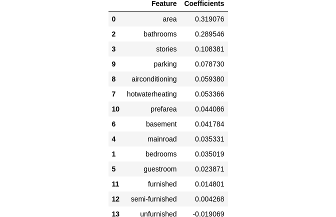

We can see that the equation of our best fitted line is:

House price = 0.31×area+0.29×bathrooms+0.10×stories +0.07×parking+……….

4. Assumption in Linear Regression

Regression is a parametric approach. Parametric means it makes assumptions about data for the purpose of analysis. Due to its parametric side, regression is restrictive in nature and cannot be applied to any regression problem, First we have to check all the assumptions stand true for linear Regression to work magically otherwise it fails to deliver good results with data sets which doesn’t fulfill its assumptions. Therefore, for a successful regression analysis, it’s essential to validate these assumptions.

Let’s look at the important assumptions in regression analysis:

4.1 Linear and Additive Relationship :

Assumption: There should be a linear and additive relationship between dependent (response) variable and independent (predictor) variable(s). A linear relationship suggests that a change in response Y due to one unit change in X¹ is constant, regardless of the value of X¹. An additive relationship suggests that the effect of X¹ on Y is independent of other variables.

Consequence: If you fit a linear model to a non-linear, non-additive data set, the regression algorithm would fail to capture the trend mathematically, thus resulting in an inefficient model. Also, this will result in erroneous predictions on an unseen data set.

Check : Look for residual vs fitted value(predicted values) plots. Also, you can include polynomial terms (X, X², X³) in your model to capture the non-linear effect. A residual plot is a graph that shows the residuals on the vertical axis and the independent variable on the horizontal axis. If the points in a residual plot are randomly dispersed around the horizontal axis, a linear regression model is appropriate for the data; otherwise, a nonlinear model is more appropriate. Below, the residual plots show three typical patterns. The first plot shows a random pattern, indicating a good fit for a linear model.

The other plot patterns are non-random (U-shaped and inverted U), suggesting a better fit for a nonlinear model.

Solution : To overcome the issue of non-linearity, you can do a non linear transformation of predictors such as log (X), √X, X² or Box-Cox power transform the dependent variable.

Python Code : Here in our House Price Prediction we can see plot shows a random pattern, indicating a good fit for a linear model. So, this assumption holds true for our problem statement.

# Code for Residual vs Fitted graph 
residuals = y_test-y_pred  
train_residuals = y_train -y_train_pred
sns.regplot(x=residuals, y=y_pred)

4.2 No AutoCorrelation :

Assumption: There should be no correlation between the residual (error) terms. Absence of this phenomenon is known as Autocorrelation.

Consequence: The presence of correlation in error terms drastically reduces model’s accuracy. This usually occurs in time series models where the next instant is dependent on previous instant. If the error terms are correlated, the estimated standard errors tend to underestimate the true standard error.
Due to this there can occur these types of problem:

Narrow confidence Interval — Narrower confidence interval means that a 95% confidence interval would have lesser probability than 0.95 that it would contain the actual value of coefficients. Let’s understand narrow prediction intervals with an example:
For example, the least square coefficient of X¹ is 15.02 and its standard error is 2.08 (without autocorrelation). But in presence of autocorrelation, the standard error reduces to 1.20. As a result, the prediction interval narrows down to (13.82, 16.22) from (12.94, 17.10).
Lower p-value of insignificant feature — lower standard errors would cause the associated p-values to be lower than actual. This will make us incorrectly conclude a parameter to be statistically significant.

Check: Look for Durbin – Watson (DW) statistic. It must lie between 0 and 4. If DW = 2, implies no autocorrelation, 0 < DW < 2 implies positive autocorrelation while 2 < DW < 4 indicates negative autocorrelation. Also, you can see residual vs time plot and look for the seasonal or correlated pattern in residual values.

Solution: If data is auto correlated then probably you can try tree based methods or time series , linear regression is not recommended.

Python Code: The autocorrelation value is 0.522 which we can consider as weakly correlated. So, this assumption holds true for our problem statement.

#  Code for durbin watson test 
from statsmodels.stats.stattools import durbin_watson
durbin_watson(y_train)0.5144520641144134

4.3 No Multicolinearity :

Assumption:The independent variables should not be correlated. Absence of this phenomenon is known as multicollinearity.

Consequences: In a model with correlated variables, it becomes a tough task to figure out the true relationship of a predictors with response variable.
These causes these problems:

Misguiding Relationship and Coefficients : When predictors are correlated, the estimated regression coefficient of a correlated variable depends on which other predictors are available in the model. If this happens, you’ll end up with an incorrect conclusion that a variable strongly/weakly affects target variable. Since, even if you drop one correlated variable from the model, its estimated regression coefficients would change. That’s not good!
Wider confidence Interval : With presence of correlated predictors, the standard errors tend to increase. And, with large standard errors, the confidence interval becomes wider leading to less precise estimates of slope parameters.
Higher p-value of significant feature — higher standard errors would cause the associated p-values to be higher than actual. This will make us incorrectly conclude a parameter to be statistically insignificant.

Check: Two methods can be used to check multicolinearity

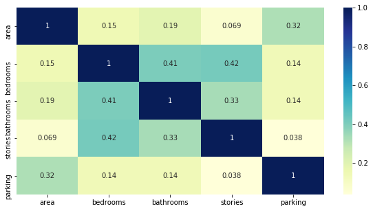
Method 1 — Correlation/Scatter plot :You can use scatter/correlation plot to visualize correlation effect among variables.
Method 2 — Variance Inflation Factor(VIF) : VIF value <= 4 suggests no multicollinearity whereas a value of >= 10 implies serious multicollinearity.

Solution: Remove all the features which are highly correlated by using Correlation/Scatter plot or Variance Inflation Factor and run linear regression taking other features. Also, regularization (Lasso(L1) and Ridge(L2)) techniques can be used in data preprocessing to handle outliers and dimensionality reduction to remove multi-collinearity for preliminary analysis.

Python Code: Using Correlation plot and VIF factor we can see multicolinear variables. From the correlation plot we can see that

# Method 1 - Correlation/Scatter plot
#  correlation to see which variables are highly correlated
numerical_cols = ['area', 'bedrooms', 'bathrooms', 'stories', 'parking']
plt.figure(figsize = (10, 5))
sns.heatmap(X_train[numerical_cols].corr(), annot = True, cmap="YlGnBu")
plt.show()## Scatter plot code
#sns.pairplot(X_train)
#plt.show()

# Method 2 - Variance Inflation Factor(VIF)
# Calculate the VIFs for the model
from statsmodels.stats.outliers_influence import variance_inflation_factor
vif = pd.DataFrame()
X = X_train[numerical_cols]
vif['Features'] = X.columns
vif['VIF'] = [variance_inflation_factor(X.values, i) for i in range(X.shape[1])]
vif['VIF'] = round(vif['VIF'], 2)
vif = vif.sort_values(by = "VIF", ascending = False)
vif

Note : Categorical variables cannot be colinear. They do not represent linear measures in Euclidean space. A chi-square test can be used to test for independence of categorical variables.

4.4 Homoskedasticity (Constant Variation) :

Assumption: The error terms must have constant variance. This phenomenon is known as homoskedasticity. The presence of non-constant variance is referred to heteroskedasticity.

Consequences: The presence of non-constant variance in the error terms results in heteroskedasticity. Generally, non-constant variance arises in presence of outliers or extreme leverage values. Look like, these values get too much weight, thereby disproportionately influences the model’s performance. When this phenomenon occurs, the confidence interval for out of sample prediction tends to be unrealistically wide or narrow.

Check:There are two ways by plot or by statistical test to test this -

Plots : Residual vs Fitted value(Predicted values) Plots shows Non-constant error variance in any of the following ways:
The plot has a “fanning” effect. That is, the residuals are close to 0 for small x values and are more spread out for large x values.

The plot has a “funneling” effect. That is, the residuals are spread out for small x values and close to 0 for large x values.Or, the spread of the residuals in the residuals vs. fits plot varies in some complex fashion.

Statistical Test : Breusch-Pagan / Cook — Weisberg test,Goldfeld-Quandt or White general test: Breusch-Pagan Lagrange/ Cook — Weisberg,Goldfeld-Quandt or White general Multiplier test for heteroscedasticity.This tests the hypothesis that the residual variance does not depend on the variables in x in the form.Homoscedasticity implies that α=0.So, Small p-value (p-val below) shows that there is violation of homoscedasticity.

Solution: To overcome heteroskedasticity, a possible way is to transform the response variable such as log(Y) or √Y. Also, you can use weighted least square method to tackle heteroskedasticity.

Python Code: We can use statsmodel package to do the following test. From the graph we are not able to clearly see homoskedasticity, but from the statistical test we can see that there is violation of homoscedasticity.

# PLOT : Code for Residual vs Fitted graph 
sns.regplot(x=residuals, y=y_pred)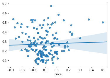

# STATISTICAL TEST: Lagrange Multiplier Heteroscedasticity Test by  # Breusch-Pagan
import statsmodels.stats.api as sms
from statsmodels.compat import lzip
name = ['Lagrange multiplier statistic', 'p-value',
        'f-value', 'f p-value']
test = sms.het_breuschpagan(train_residuals,X_train)
lzip(name, test)[('Lagrange multiplier statistic', 52.253243690033884),
 ('p-value', 1.2182517345931792e-06),
 ('f-value', 4.48719032464496),
 ('f p-value', 4.1478253819674125e-07)]name = ['F statistic', 'p-value']
test = sms.het_goldfeldquandt(train_residuals,X_train)
lzip(name, test)[('F statistic', 1.2641511162146375), ('p-value', 0.06016643261192988)]# STATISTICAL TEST: White’s Lagrange Multiplier Test for            # Heteroscedasticity.
test = sms.het_white(train_residuals,X_train)
lzip(name, test)[('F statistic', 204.6884831288231), ('p-value', 3.373894291207971e-10)]

4.5 Normal Distribution of error terms :

Assumption:The error terms must be normally distributed.

Consequences:If the error terms are non- normally distributed, confidence intervals may become too wide or narrow. Once confidence interval becomes unstable, it leads to difficulty in estimating coefficients based on minimization of least squares.

Check: There are two ways by plot or by statistical test to test this-

Plots : QQ plot QQ or quantile-quantile is a scatter plot which helps us validate the assumption of normal distribution in a data set. Using this plot we can infer if the data comes from a normal distribution. If yes, the plot would show fairly straight line. Absence of normality in the errors can be seen with deviation in the straight line.

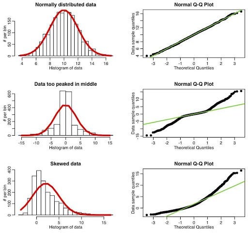
Statistical Test — Jarque-Bera test, Omni test, Kolmogorov-Smirnov test or Shapiro-Wilk test The null hypothesis for the test is that the data is normally distributed; the alternate hypothesis is that the data does not come from a normal distribution.So, Small p-value (pval below) shows that residuals are normally distributed.

Solution: If the errors are not normally distributed, non – linear transformation of the variables (response or predictors) can bring improvement in the model.

Python Code: Form the plot we can say that residuals are normally distributed and test also confirms that

# PLOT : Code for QQ Plot
import pylab as py 
import statsmodels.api as sm 
sm.qqplot(train_residuals, line ='45') 
py.show()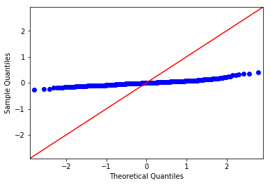

# STATISTICAL TEST:  Jarque-Bera test
name = ['Jarque-Bera', 'Chi^2 two-tail prob.', 'Skew', 'Kurtosis']
test = sms.jarque_bera(train_residuals)
lzip(name, test)[('Jarque-Bera', 131.59921802835424),
 ('Chi^2 two-tail prob.', 2.6521183092250006e-29),
 ('Skew', 0.7620599505841854),
 ('Kurtosis', 5.442697903616747)]# STATISTICAL TEST:  Omni test
name = ['Chi^2', 'Two-tail probability']
test = sms.omni_normtest(train_residuals)
lzip(name, test)[('Chi^2', 56.9510496636162), ('Two-tail probability', 4.2977059361473576e-13)]# STATISTICAL TEST: Kolmogorov-Smirnov test 
import scipy
scipy.stats.kstest(train_residuals, 'norm')KstestResult(statistic=0.4162251367016485, pvalue=0.0)# STATISTICAL TEST: Shapiro-Wilk test
shapiro_test=scipy.stats.shapiro(train_residuals)
shapiro_test(0.9591060280799866, 8.284670727221055e-09)

5. Regression Metrics to evaluate the Model

Given our Simple Linear Regression equation:

Y = bX + a

We can use the following Metrics to find the coefficients:

5.1 Mean Absolute Error (MSE)

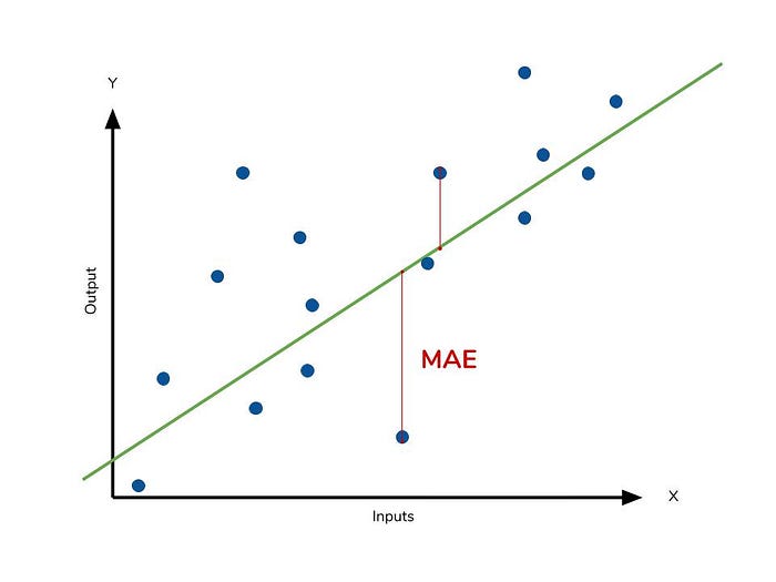
MAE is the absolute difference between the target value and the value predicted by the model. The MAE is more robust to outliers and does not penalize the errors as extremely as MSE. MAE is a linear score which means all the individual differences are weighted equally. It is not suitable for applications where you want to pay more attention to the outliers.

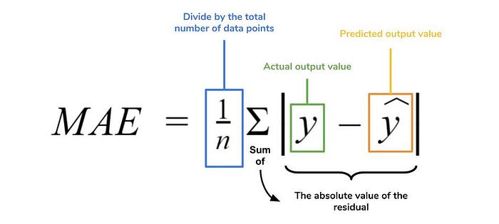
The picture below is a graphical description of the MAE. The green line represents our model’s predictions, and the blue points represent our data. MAE

5.2 Mean Squared Error (MSE)

MSE or Mean Squared Error is one of the most preferred metrics for regression tasks. It is simply the average of the squared difference between the target value and the value predicted by the regression model. As it squares the differences, it penalizes even a small error which leads to over-estimation of how bad the model is. It is preferred more than other metrics because it is differentiable and hence can be optimized better.

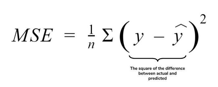
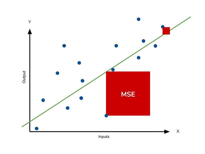
This is to say that large differences between actual and predicted are punished more in MSE than in MAE. The following picture graphically demonstrates what an individual residual in the MSE might look like.

5.3 Root Mean Squared Error:

RMSE is the most widely used metric for regression tasks and is the square root of the averaged squared difference between the target value and the value predicted by the model. It is preferred more in some cases because the errors are first squared before averaging which poses a high penalty on large errors. This implies that RMSE is useful when large errors are undesired.Because the MSE is squared, its units do not match that of the original output. Researchers will often use RMSE to convert the error metric back into similar units, making interpretation easier.

The following picture graphically demonstrates what an individual residual in the MSE might look like and summation of all points followed by square root gives us RMSE

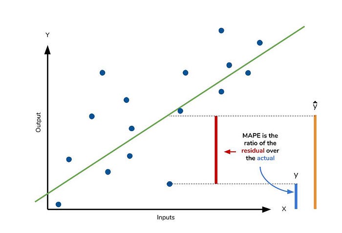
5.4 Mean Absolute Percentage Error:

The mean absolute percentage error (MAPE) is the percentage equivalent of MAE. The equation looks just like that of MAE, but with adjustments to convert everything into percentages.

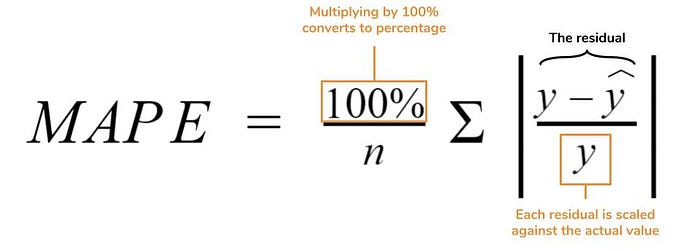
Like MAE, MAPE also has a clear interpretation since percentages are easier for people to conceptualize. Both MAPE and MAE are robust to the effects of outliers thanks to the use of absolute value.MAPE has disadvantage i.e it is undefined for data points where the value is 0. Similarly, the MAPE can grow unexpectedly large if the actual values are exceptionally small themselves.

5.5 Mean Percentage Error:

The mean percentage error (MPE) equation is exactly like that of MAPE. The only difference is that it lacks the absolute value operation.While the absolute value in MAPE eliminates any negative values, the mean percentage error incorporates both positive and negative errors into its calculation.

Since positive and negative errors will cancel out, we cannot make any statements about how well the model predictions perform overall. However, if there are more negative or positive errors, this bias will show up in the MPE. Unlike MAE and MAPE, MPE is useful to us because it allows us to see if our model systematically underestimates (more negative error) or overestimates (positive error).

5.6 R² Error:

Coefficient of Determination or R² is another metric used for evaluating the performance of a regression model. The metric helps us to compare our current model with a constant baseline and tells us how much our model is better. The constant baseline is chosen by taking the mean of the data and drawing a line at the mean. R² is a scale-free score that implies it doesn’t matter whether the values are too large or too small, the R² will always be less than or equal to 1.

The Graph shows the visual interpretaion of R²

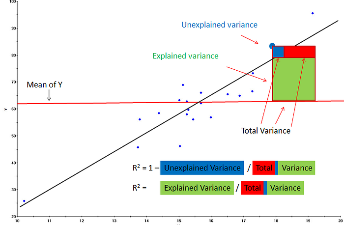
Note: R² can be negative,the main reason for R² to be negative is that the chosen model does not follow the trend of the data causing the R² to be negative. This causes the mse of the chosen model(numerator) to be more than the mse for constant baseline(denominator) resulting in negative R².

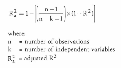
5.7 Adjusted R²:

Adjusted R² depicts the same meaning as R² but is an improvement of it. R² suffers from the problem that the scores improve on increasing terms even though the model is not improving which may misguide the researcher. Adjusted R² is always lower than R² as it adjusts for the increasing predictors and only shows improvement if there

6. Advantages and Disadvantages of Linear Regression

6.1 Advantages

Simple model : The Linear regression model is the simplest equation using which the relationship between the multiple predictor variables and predicted variable can be expressed.The mathematical equations of Linear regression are also fairly easy to understand and interpret.Hence Linear regression is very easy to master.
Computationally efficient : Linear regression has a considerably lower time complexity when compared to some of the other machine learning algorithms i.e. modeling speed of Linear regression is fast as it does not require complicated calculations and runs predictions fast when the amount of data is large.
Interpretability of the Output: The ability of Linear regression to determine the relative influence of one or more predictor variables to the predicted value when the predictors are independent of each other is one of the key reasons of the popularity of Linear regression. The model derived using this method can express what change in the predictor variable causes what change in the predicted or target variable.
Overfitting can be reduced by regularization: Overfitting is a situation that arises when a machine learning model fits a dataset very closely and hence captures the noisy data as well.This negatively impacts the performance of model and reduces its accuracy on the test set.

Regularization is a technique that can be easily implemented and is capable of effectively reducing the complexity of a function so as to reduce the risk of overfitting

6.2 Disadvantages

Prone to underfitting : Underfitting : A situation that arises when a machine learning model fails to capture the data properly.This typically occurs when the hypothesis function cannot fit the data well.
Prone to noise and overfitting: If the number of observations are lesser than the number of features, Linear Regression should not be used, otherwise it may lead to overfit because is starts considering noise in this scenario while building the model.
Sensitive to outliers : Outliers of a data set are anomalies or extreme values that deviate from the other data points of the distribution.Data outliers can damage the performance of a machine learning model drastically and can often lead to models with low accuracy.Outliers can have a very big impact on linear regression’s performance and hence they must be dealt with appropriately before linear regression is applied on the dataset.
Limited use due to several Assumption: If all the assumptions as discussed above are not met then Linear Regression might be not the right choice

Linear and Additive Relationship
No AutoCorrelation
No Multicolinearity
No Heteroskedasticity
Normal Distribution of error terms

If assumptions are not met then the coefficient from regression could be misleading and leads to bad predictions

Summary

Linear Regression is a great tool to analyze the relationships among the variables but it isn’t recommended for most practical applications because it over-simplifies real-world problems by assuming a linear relationship among the variables.Before applying Linear Regression all the assumption should be checked and Model can be evaluated using different metrics based on particular problem statement and its objective.

Sources Used

Footnotes

I know this was a long one. But, the most important one too!. I hope you are learning. Please ping me on linkedin if you have any suggestions or correction.

Thanks for reading. 🙂
And, ❤️ if this was a good read. Enjoy!